Recent Posts
Rambles in Machine Learning
21. February, 2019
Classifying Chatrooms with scikit-learn
Machine Learning has been ascending in the Zeitgest for long enough that I'm probably behind the curve, but that wasn't going to prevent me from having a shoofty (apparently the most common spelling is "shufti" but never mind). Since python has been my programming home since at least 2009, scikit-learn was the obvious choice of tool. (unfortunately my projects folder's metadata got nuked during a file-transfer in 2009. Looking through now, my earliest verifiable python project was pyGenes, a Creatures 3 genome editor, which existed by 2005!)
Last year I bought Introduction to Machine Learning with Python along with a bunch of other Machine Learning books as part of a humble bundle, and had already read through it (though without actually writing any code myself... an activity which may be of questionable value) so I had a reasonable idea of what kind of toolkit it was. Having had the idea to attempt some ML project back then the key question was of course what I could investigate.
I didn't want to just play with the included data --- something done to death and quite boring, no matter how cool training handwriting classifiers on MNIST is (and anyway, you do this in coursera's Machine Learning course). But there are very few datasets that one already has that are suitable for the task, especially when one considers that I am far too lazy to hand-label more than about ten lines of data before getting bored and giving up. Unsupervised learning is always a possibility, but it lacks easily-quantifed metrics of success and there is the very real risk that you need genuine insight and intelligence to do something interesting. I thought about collecting League of Legends data and deriving stats and strategies from that... but many people are doing this already, probably much better than me and then I finally followed the advice of all my teammates over the years and uninstalled the game, so I also lost the personal interest.
Thankfully, a trusty piece of technology invented in the year of my birth came to the rescue: IRC. Thanks to Quassel I have chatroom logs dating back to 2012: millions of lines from thousands of people, all ready-labeled with all sorts of metadata and in a convenient Postgres database. Even my discord chats are routed through Quassel using bitlbee (I refuse to come back to Slack now they killed off the IRC transport) My first idea: predicting from lines of chat which chatroom it was said in. This already offers a bunch of routes of exploration in terms of pre-processing, model selection and tuning, and is just the kind of supervised Natural Language Processing classification task that people have been doing for ages.
In fact the scikit-learn documentation has a tutorial on text data which covers exactly this kind of scenario, only classifying BBS posts into their newsgroups instead of IRC messages into channels. Before I discovered this I had been fiddling around with textacy, but the key feature I needed from textacy for the initial experiments was a vectorizer (transforming text into a sparse array where a[i] = n means that there were  occurrences of the word with index
  in some enumeration of words) and it turns out scikit-learn itself contains some options for this.
So for this initial project I set the following parameters:
-
Attempt to classify which of five IRC/Discord channels lines of text came from
-
Use scikit-learn's
SGDClassifier(i.e. an SVM) since that's what the tutorial does -
Use a grid-search to find some decent parameters
-
Remove nicknames from the text
The last one was something I decided I wanted to do early on --- if IRCUser42 is only present in #channel1, then any line that happens to be directly addressed to her (or mentions her name) will of course be easy to classify. We want to set the model a challenge!
Here's the code I used to train the model and print some statistics about it:
import numpy as np
from sklearn.feature_extraction.text import CountVectorizer
from sklearn.model_selection import train_test_split, GridSearchCV
from sklearn.linear_model import SGDClassifier
from sklearn.preprocessing import StandardScaler
from sklearn.pipeline import Pipeline
from sklearn import metrics

def train(data, labels, nicks):
    vectorizer = CountVectorizer(ngram_range=(1,3))
    tokenize = vectorizer.build_tokenizer()
    preprocess = vectorizer.build_preprocessor()
    stop_words = set()
    for n in nicks:
        stop_words |= set(tokenize(preprocess(n)))
    vectorizer.stop_words = stop_words

    tfidf = sklearn.feature_extraction.text.TfidfTransformer()
    scaler = StandardScaler(with_mean=False)
    classifier = SGDClassifier(penalty='l1', alpha=0.002, random_state=43, max_iter=5)
    pipeline = Pipeline([
        ('vect', vectorizer),
        ('tfidf', tfidf),
        ('scaler', scaler),
        ('clf', classifier)])
    parameters = {
        'vect__ngram_range': [(1,1),(1,2),(1,3)],
        'tfidf__use_idf': (True, False),
        'clf__alpha': (1e-1, 1e-2, 1e-3),
        'clf__penalty': ('l1', 'l2')
    }
    #if cv is low, best_score_ will be low, but the training/test scores may still be high.
    search = GridSearchCV(pipeline, parameters, cv=3, iid=True, n_jobs=-1)

    X_train, X_test, y_train, y_test = train_test_split(data, labels, random_state=43, stratify=labels)
    #model.fit(X_train, list(y_train))

    model = search.fit(X_train, y_train)
    print('Best parameters:', model.best_params_)
    print('Best CV score: %.2f' % (model.best_score_))
    print('Training score: %.2f' % (model.score(X_train, y_train)))
    print('Test score: %.2f' % (model.score(X_test, y_test)))
    predicted = model.predict(X_test)
    print(metrics.classification_report(y_test, predicted))
    print(metrics.confusion_matrix(y_test, predicted))

    return model
```
data and labels should be the lines of chat and channel names, which can be obtained from Quassel's backlog database, as numpy arrays. nicks should be a list of nicknames to filter from the text. We just use the Vectorizer's stop_words attribute for this so we could use this to filter out anything. It's worth pointing out that many nicknames are real English words. It would be crazy to filter those out, so when generating the list of nicks, we throw out anything in an English vocabulary list. This is the only bit of the process which is language-dependent.
I run the model like this:
>>> train(rows[:,0], rows[:,1], nicks)
    Best parameters: {'tfidf__use_idf': True, 'clf__alpha': 0.01, 'clf__penalty': 'l2', 'vect__ngram_range': (1, 1)}
    Best CV score: 0.54
    Training score: 0.76
    Test score: 0.56
                       precision    recall  f1-score   support

    #Ins.general-chat       0.57      0.47      0.51      1000
    #Str.general-chat       0.56      0.45      0.50      1000
               #latex       0.64      0.70      0.67      1000
             #notpron       0.46      0.56      0.51      1000
             #quassel       0.57      0.61      0.59      1000

            micro avg       0.56      0.56      0.56      5000
            macro avg       0.56      0.56      0.56      5000
         weighted avg       0.56      0.56      0.56      5000

    [[470 128  76 207 119]
     [164 449  69 212 106]
     [ 39  45 705 102 109]
     [101 120 102 556 121]
     [ 56  60 151 119 614]]
A null model which just guessed one class all the time would score 20% so this isn't too bad, but it isn't great, either. It's worth noting that since the classes are (almost) equal in size, the accuracy score is a reasonable summary metric. It's no more important to correctly classify lines from #latex as coming from #latex than it is to, say, avoid incorrectly labelling lines as coming from #quassel. I was surprised that the grid search found that ngrams were worse than bags of words for accuracy. This means that the model was best able to learn purely from the vocabulary used in the different channels, and not from the patterns of words at all.
Let's look at the confusion matrix visually:
import matplotlib.pyplot as plt

def plot_confusion_matrix(cm, classes):
    cm_norm = cm.astype('float')/cm.sum(axis=1)[:, np.newaxis]
    cmap = plt.cm.get_cmap('Blues')
    plt.imshow(cm, interpolation='nearest', cmap=cmap)
    plt.colorbar()
    plt.title('Confusion Matrix of SVM')
    plt.xlabel('Prediction')
    plt.ylabel('Channel')
    tick_marks=np.arange(len(classes))
    plt.xticks(tick_marks, classes, rotation=20, ha='right')
    plt.yticks(tick_marks, classes)
    import itertools
    for i, j in itertools.product(range(cm.shape[0]), range(cm.shape[1])):
        plt.text(j, i, cm[i, j], ha='center', color='white' if cm_norm[i,j] > 0.5 else 'black')
    plt.tight_layout()
Running this gives us:
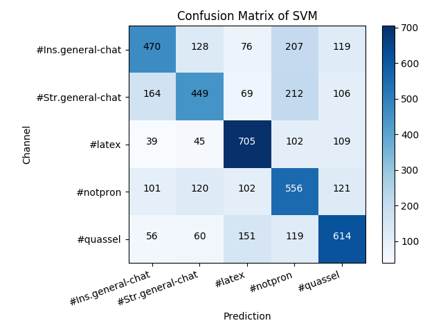
From this we can easily see where the model did badly and where it did better. #latex and #quassel were the easiest to classify — no surprise since they are technical support channels with the attendant unique jargon. The other three channels are general chat channels and harder to distinguish. #Ins.general-chat and #Str.general-chat in particular are both video game focused with overlapping user bases, so the fact they were the hardest to classify is also not surprising, but it's worth pointing out that they were both mis-labeled more often as #notpron than as each other, which is odd. While the two general-chats were less often mis-labeled as #latex, #quassel was more often, presumably because of general tech support vocab.
How can we improve the accuracy? An easy way would be to make the problem easier! Something you don't always have the luxury of doing but while playing around, why not. Reducing the number of classes makes things a lot easier — classifying between two channels got over 70% accuracy with no tuning. But this is pretty boring. On the other hand it's not unreasonable to feed the model more data at a time by concatenating several lines of chat. We can do this with the same data from the database as before, contained in rows:
def chunks(l, n):
    for i in range(0, len(l), n):
        yield l[i:i + n]

joined = []
joined_label = []
for rr, l in zip(chunks(rows[:,0], 4), rows[:,1][::4]):
    joined.append('\n'.join(rr))
    joined_label.append(l)
Rerunning train gives us a test score of 63%, a marked improvement — especially since we didn't actually give the model any more data, just fed it more at once. If we instead retrieve more rows from the database to jam together, say 25,000 from each channel and stick together 5 at once, we get the following parameters and scores:
Best parameters: {'tfidf__use_idf': True, 'clf__alpha': 0.001, 'clf__penalty': 'l2', 'vect__ngram_range': (1, 1)}
Best CV score: 0.74
Training score: 0.86
Test score: 0.76
                   precision    recall  f1-score   support

#Ins.general-chat       0.80      0.53      0.64       753
#Str.general-chat       0.77      0.70      0.73      1247
           #latex       0.76      0.95      0.84      1250
         #notpron       0.74      0.65      0.69      1250
         #quassel       0.75      0.88      0.81      1250

        micro avg       0.76      0.76      0.76      5750
        macro avg       0.76      0.74      0.74      5750
     weighted avg       0.76      0.76      0.75      5750

[[ 399  133   47  102   72]
 [  62  875   57  143  110]
 [   1    7 1182   12   48]
 [  30  107  164  810  139]
 [   6   17  100   24 1103]]
Oops, it looks like there weren't that many qualifying lines from the first two channels, though overall we are doing much better. A null model here would still only get an accuracy of 22%. You can see that the model hardly misclassifies anything as #Ins.general-chat (best precision) but misclassifies it as other things more frequently than any other channel. Nevertheless the recall is slightly improved compared to the situation with equal classes and less data. Let's visualise the confusion matrix again (normalised to the support):
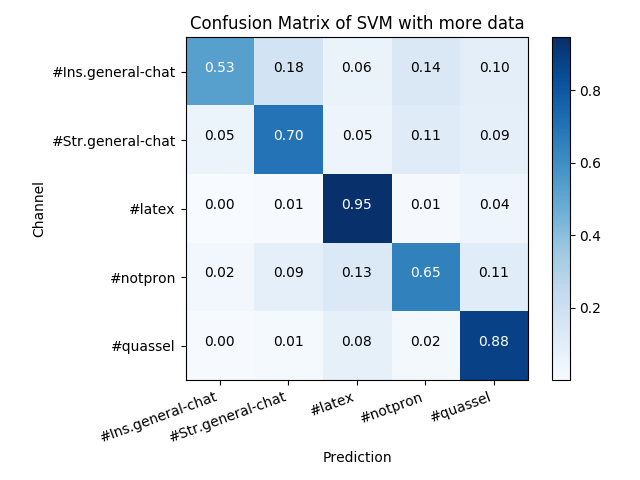
The cross-validation is still finding that ngrams don't help. This does mean that we can easily examine what are the most important words for classification. The SVM stores its coefficients under the coef_ parameter and we can get an idea of which words the model thinks are associated with being in - or not being in - each category by whether the corresponding coefficient is strongly positive or strongly negative. We use numpy.argsort to return the indices of the largest coefficients, and retrieve the associated word from the vectoriser with get_feature_names()[index].
# Retrieve the vectoriser and SVM portions of the pipeline
vec = model.best_estimator_.steps[0][1]
svm = model.best_estimator_.steps[3][1]
# Retrieve the relation from vector --> word
rev = vec.get_feature_names()
for i, c in enumerate(model.classes_):
    sig = np.argsort(svm.coef_[i,:])[-25:]
    words = [rev[n] for n in sig]
    print(c)
    print("    " + " ".join(words))
#Ins.general-chat:
    picker hyped beans minutes i65 seat expo 26th 289695103902285824 clan 30 i64 tickets loyalty 2019 remaining cooldown 64 byoc months mere 18th hello 22nd insomnia
#Str.general-chat:
    blur roast liab grandstand warranty paddock car fileserver attachments prop heating 448872115081314314 announcement dinner pudding pinned boiler tomorrow stratlan racecourse supcom kitchen ayce golf 266234897633509376
#latex:
    inside math environments file stackexchange page xetex section pdflatex xelatex pdf org begin paste pastebin environment texlive sample aborts package ctan compiles align document latex
#notpron:
    face riddle kinder silly wind trivia song coverage doctor humidity bgsound blowing mbar apartment country egg weather views university lounge fish finland trump url2title swedish
#quassel:
    notification version bugs windows saint connecting connection channels database messages postgresql notifications quasselsuche build builds user backlog connect quasselcore sqlite quasseldroid clients protocol client core
A couple of things are obvious from this analysis: firstly, the long numbers. Some of these come from bitlbee (failing to) render discord roles so that "@Staff" turns into a long identification number for the "Staff" role. Others come from common URL components that discord re-hosts images under. It's tricky to know the best way to deal with these - on the one hand it seems to be cheating to use some computer-generated unique identifiers. On the other, filtering out URLs - or numbers - entirely seems over the top.
"url2title" under #notpron is a label that a bot in the channel uses when it automatically prints the titles of webpages participants link. This is therefore not representative of the human participation in the channel, and an enhancement could involve filtering out bots' messages. In that channel users can also type "!weather <location>" (the source of "weather" in the list) to receive weather information from the bot, which is the source of many words there. Some words in other channels also come from bots and bot triggers.
I chose not to lemmatise the words before training because I thought that different grammar patterns in different channels might help distinguish them. In a few cases this does seem to be the case, but mostly not. Here is an example where it makes a difference:
>>> svm.coef_[:,vec.vocabulary_.get('train')]
array([ 0.00082995, -0.00049029, -0.00435588,  0.00564122, -0.00626548])

>>> svm.coef_[:,vec.vocabulary_.get('training')]
array([-0.00259072,  0.00241011, -0.00315301,  0.00380725, -0.00373427])
We see that the importance of the word flips in two cases, as well as changing a bit in others. The effect here is stronger than in most cases I checked, presumably because "training" is a completely different meaning from "a train." Rather than picking up different grammar, not lemmatising allows us to detect different meanings of words that might be squashed otherwise.
One last comment is that the #latex list is full of non-English jargon like "xetex" and "texlive," and even the real English words will be familiar to LaTeX users as being keywords in the language. Real language is littered with words that aren't in the dictionary, whether typos, slang or local jargon and it's not really possible to clean this up without removing the essential character of the chat.
All these factors affect my perception of the "fairness" of the exercise - a vague sense that when setting yourself a learning exercise you shouldn't make it too easy. Still, they are difficult to mitigate and don't really defeat the purpose.
NetHack statistics
27. October, 2013
I've recently been playing NetHack on the nethack.alt.org server and was wondering how likely you are to ascend depending on how long you survive. If you don't know, NetHack is a notoriously difficult game, and few people ever beat it (or "ascend" as it's known.) However, the greatest difficulties occur in the early game, when not just mistakes will get you killed, but also the foibles of the Random Number Generator (or the Random Number God as s/he is sometimes called.) So with the help of nethack.alt.org's extended log, documenting over 2.3 million plays of the game, ipython and matplotlib, I cooked up the following graph:
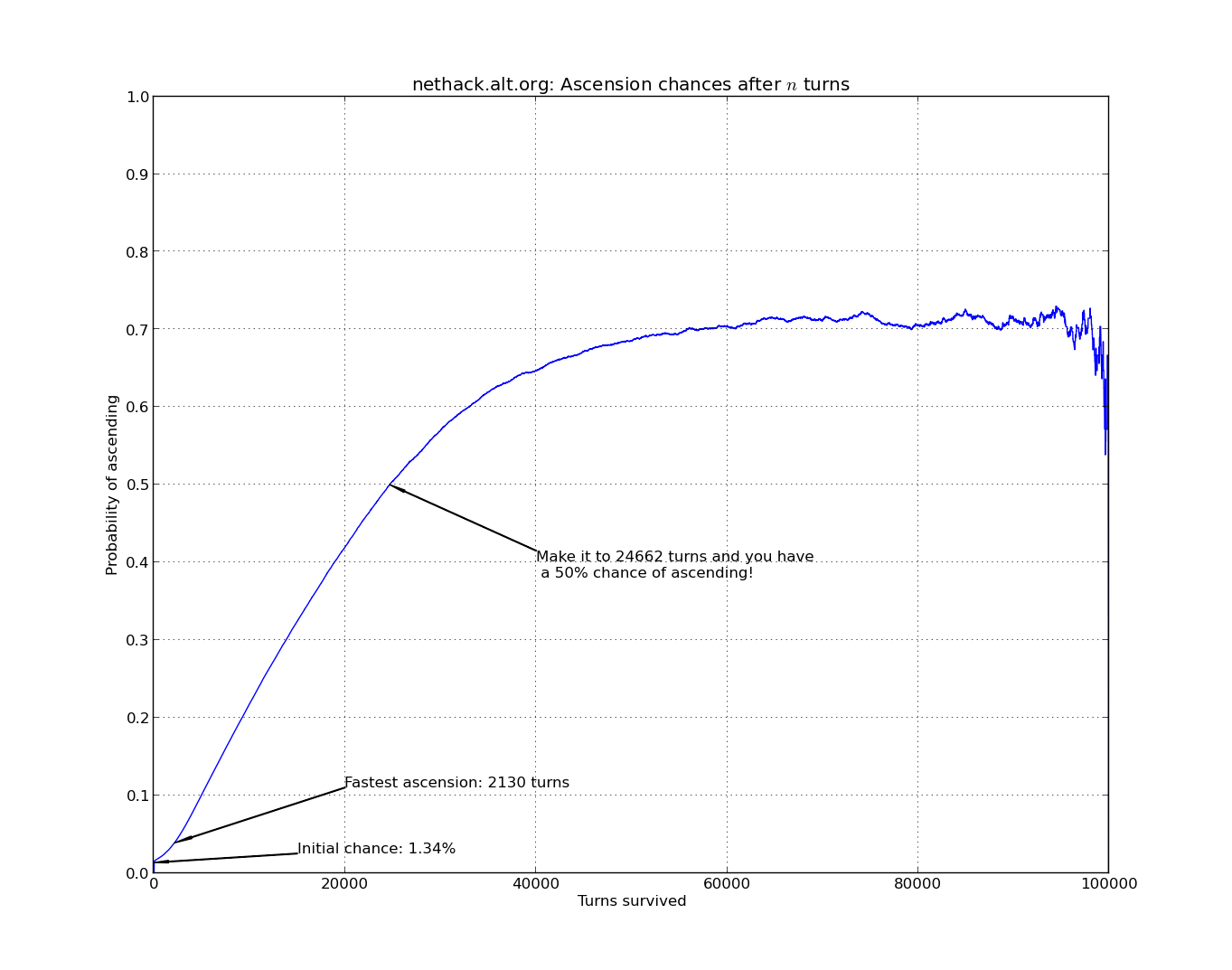
This graph shows your chance of ascending based on how long you survive in the dungeon, clearly demonstrating that the longer you survive, the better your chances. Notice though, that it never gets that certain: no matter how long you survive, it's possible to fall from glory (or, "Splat".) As the turns go on, fewer and fewer people have survived without already ascending, and the graph gets jagged and unreliable.
But what exactly is happening to our 2.3 million adventurers over the 100,000 turns graphed here? Time for more graphs:

On the left, we see the number of players dying, quitting or ascending on each turn, on two different scales: Firstly at a large scale (but still not nearly including the vast numbers of people who quit or die immediately!) for the first 5,000 turns and then zoomed in up to 50,000 turns. Both graphs have been smoothed. Note that of the 920,000 "deaths" on the first turn, almost all are due to escaping the dungeon.
On the right, we look at how many players there are of each status (alive, ascended, dead, quit) after a number of turns. On the first graph you can see that the tiny quantity of ascensions barely even features, while in the zoomed-in graph you can see how the ascensions begin to accumulate. Since many many people quit on the first turn (either by #quitting or escaping) we have excluded them from these graphs.
Here's the code I used to gather statistics on the xlogfile:
import re
from numpy import *

def movingaverage(interval, window_size):
    window = ones(int(window_size))/float(window_size)
    return convolve(interval, window, 'same')

l = 100000
r = re.compile(':death=(?P<death>[^:]+).*:turns=(?P<turns>[0-9]+)')
total = 2361141 #Total number of records with extended data available

def parse():
    global dies, quits, asc, alive, alive_asc, alive_asc_quit
    dies = [0] * l
    quits = [0] * l
    asc = [0] * l

    for line in open('xlogfile.full.txt', 'r'):
        m = r.search(line)
        if m:
            turns = int(m.group('turns'))
            if turns >= l:
                continue
            if m.group('death') == 'quit':
                quits[turns] += 1
            elif m.group('death') != 'ascended':
                dies[turns] += 1
            else:
                asc[turns] += 1

cumtotal = total - dies[1] - quits[1]
alive_asc_quit = cumtotal - cumsum(dies[2:])
alive_asc = alive_asc_quit - cumsum(quits[2:])
alive = alive_asc - cumsum(asc[2:])
Now back to 'hacking!